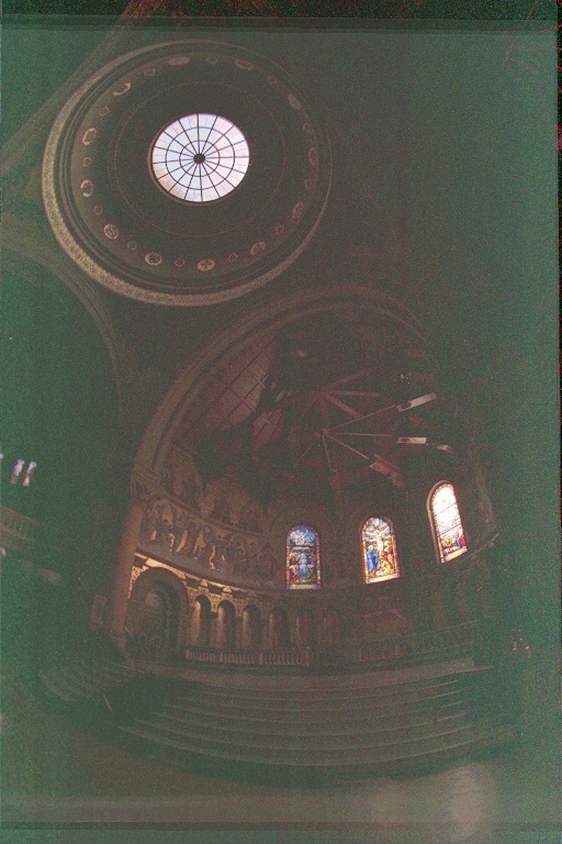
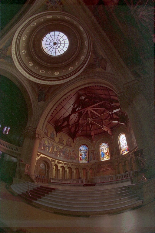
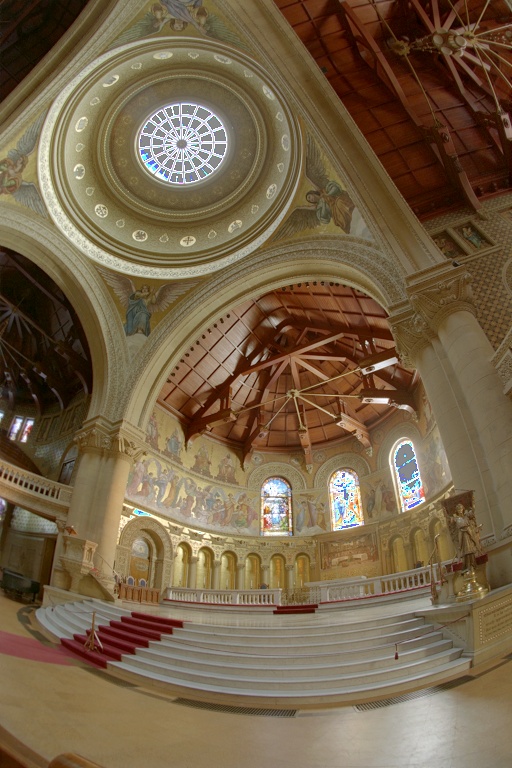
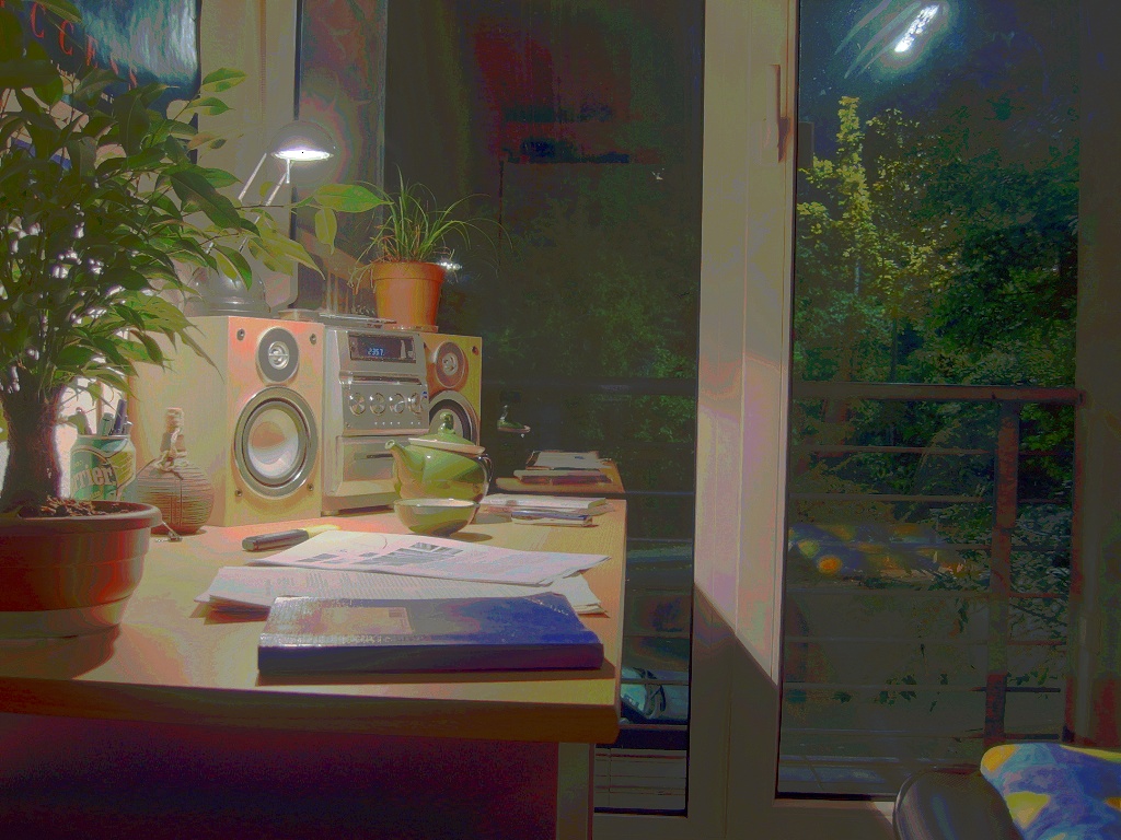
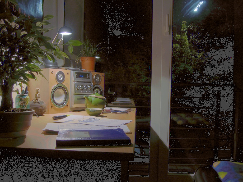
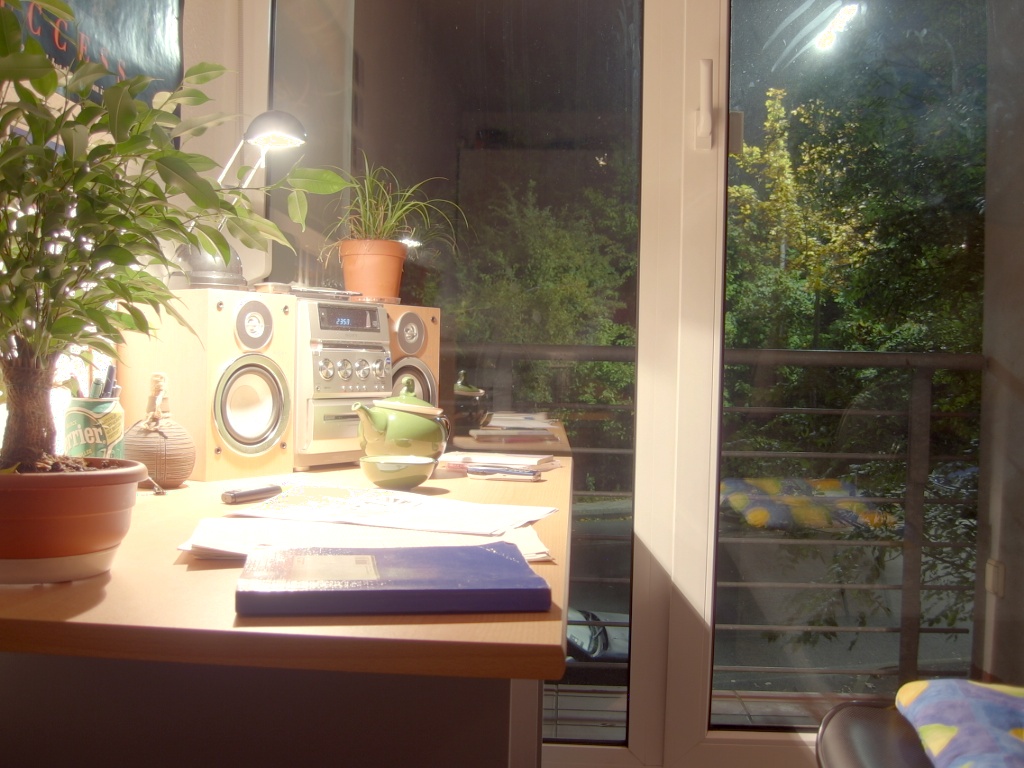
This project is to use a bunch of LDR images under different exposures to recover the radiance map and then construct a HDR image. Different construction algorithms are implemented and compared.

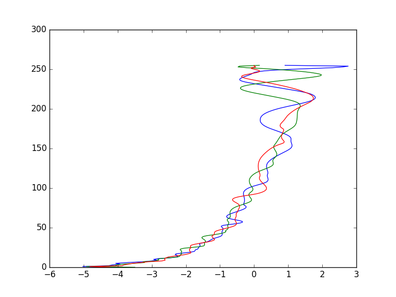
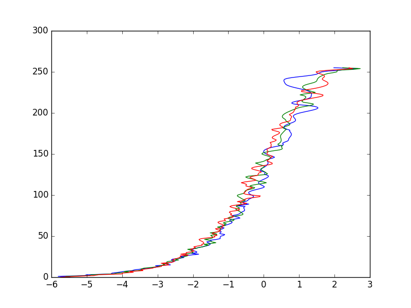
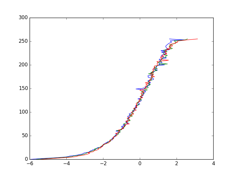
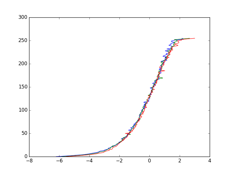
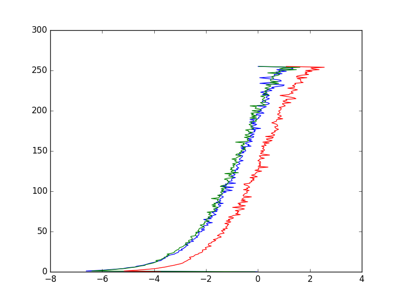
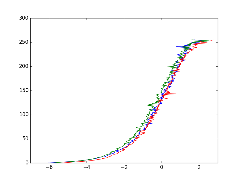
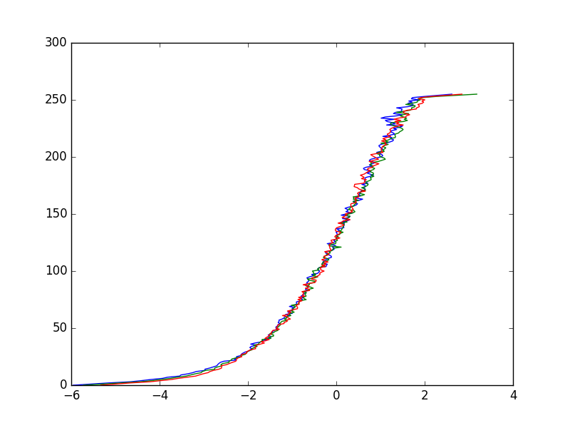
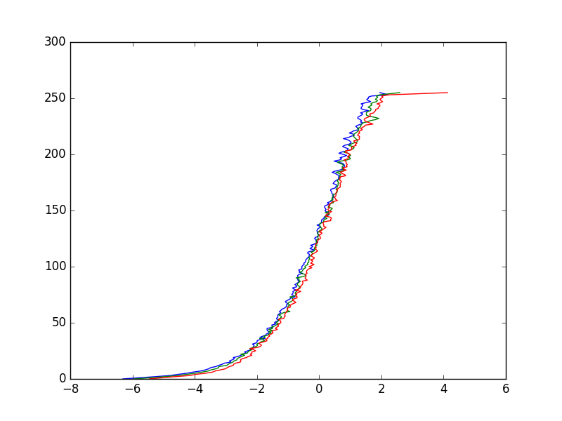
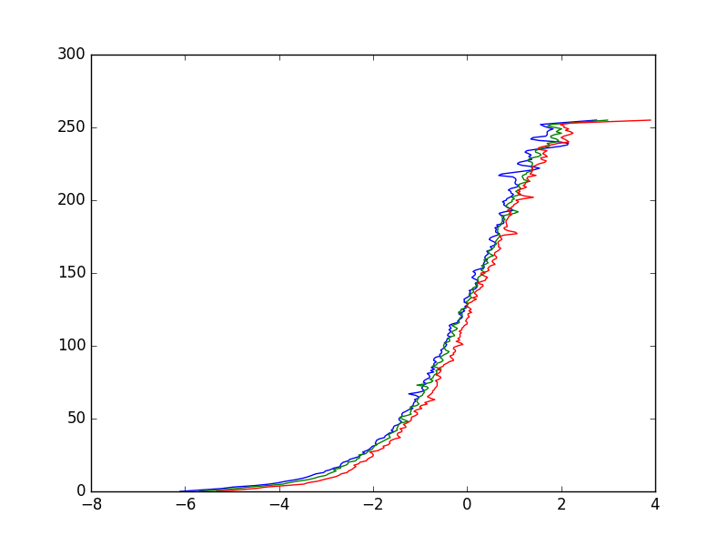
To construct a HDR image, we need to recover the radiance map first, which is a function mapping real-world radiance values to RGB values between 0 and 255. Using a bunch of images under different exposures, we know that, for each pixel, the radiance value is constant through the images, but only exposure time is changing, resulting in different RGB values. Therefore, we can select a bunch of pixels and use their constant radiance value and different RBG values in different images to construct the map from radiance values to RGB values. Here, we randomly select N pixels for R/G/B channel respectively. To smooth the curve, we add a smooth term with parameter lamda. Seen from the maps below, we can clearly see that the curve becomes smoother as N increase. More pixels are needed, however, as the pixels are randomly selected and the result can be very unstable if too few pixels are selected. And as lamda increases, the curve first becomes more smooth but then less smooth. (All the radiance maps are recovered based on the nine pictures above)

N = 10	N = 50	N = 100
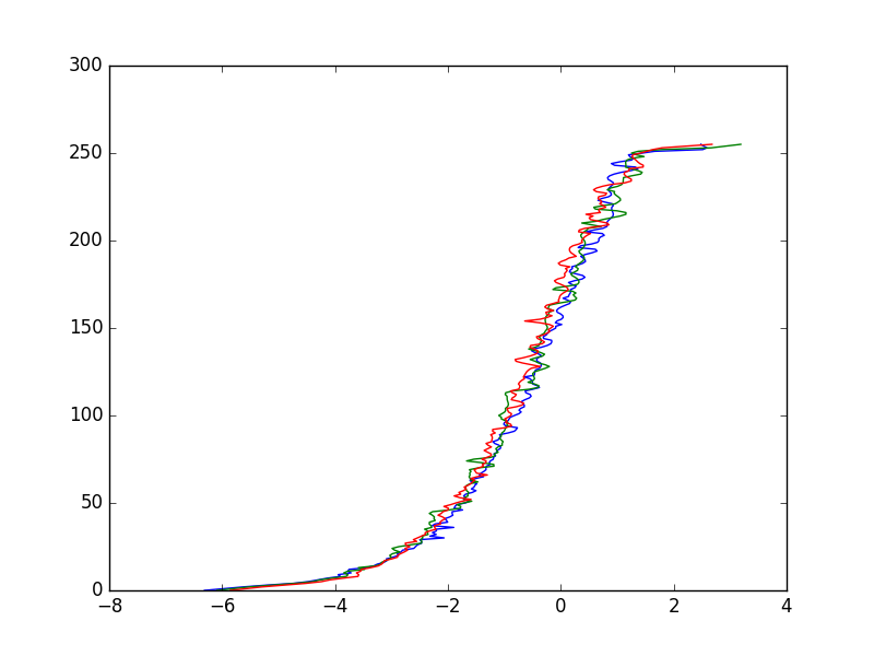N = 200	N = 300	N = 500

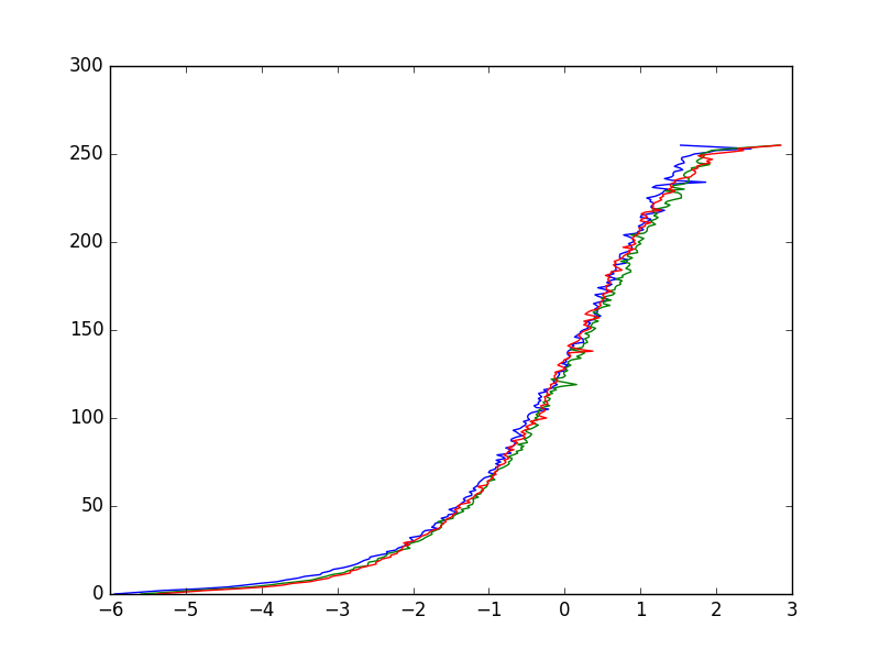lamda = 0.001	lamda = 0.01	lamda = 0.1
lamda = 0.2	lamda = 0.3	lamda = 0.4

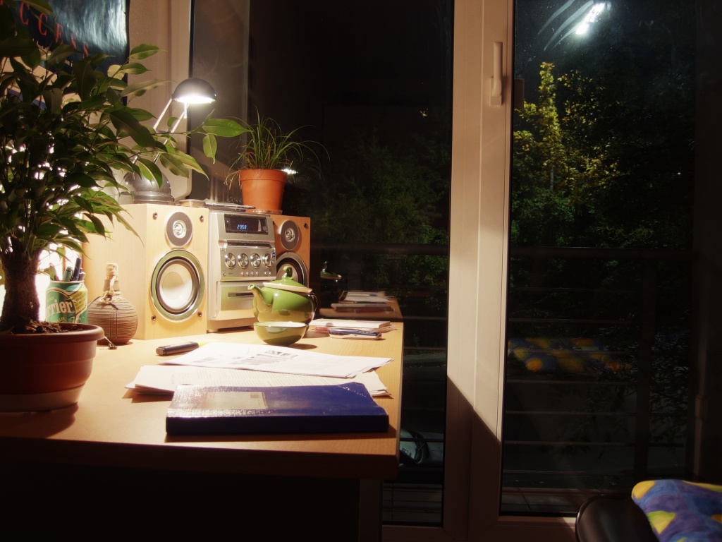
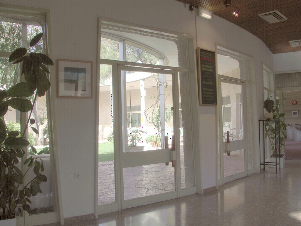
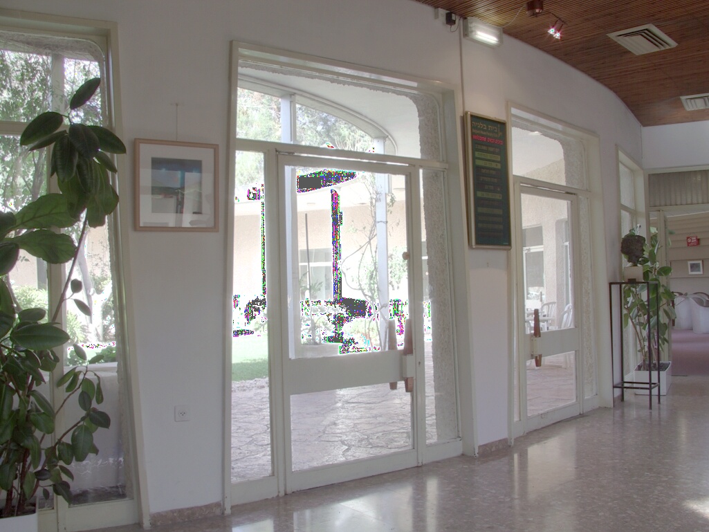
After we get the radiance map curve, we can easily calculate the real radiance value for each pixel. However, these values need to be mapped to the interval [0, 255] so that it can be stored as a digital image. One way to do so is to use some simple global operators, like L/(1+L), log(L) and so on. In some case, these operators appear to work well but generally the results are not that satisfying. Many details are missing or unclear, especially for the bright regions.

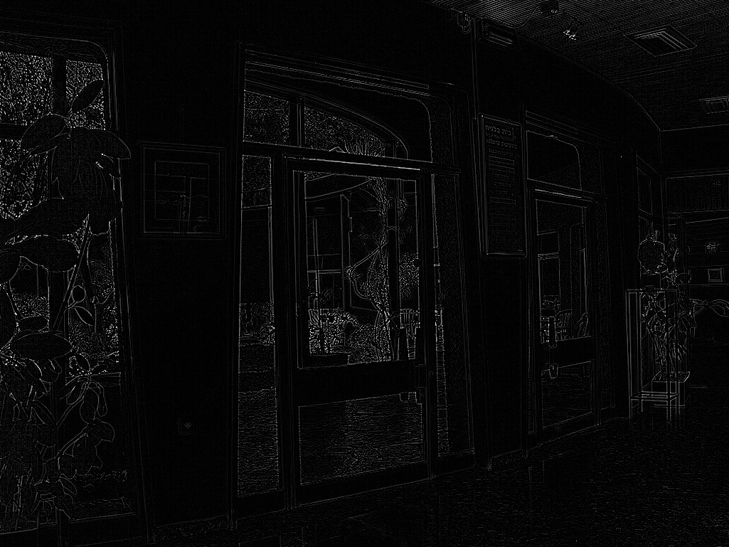
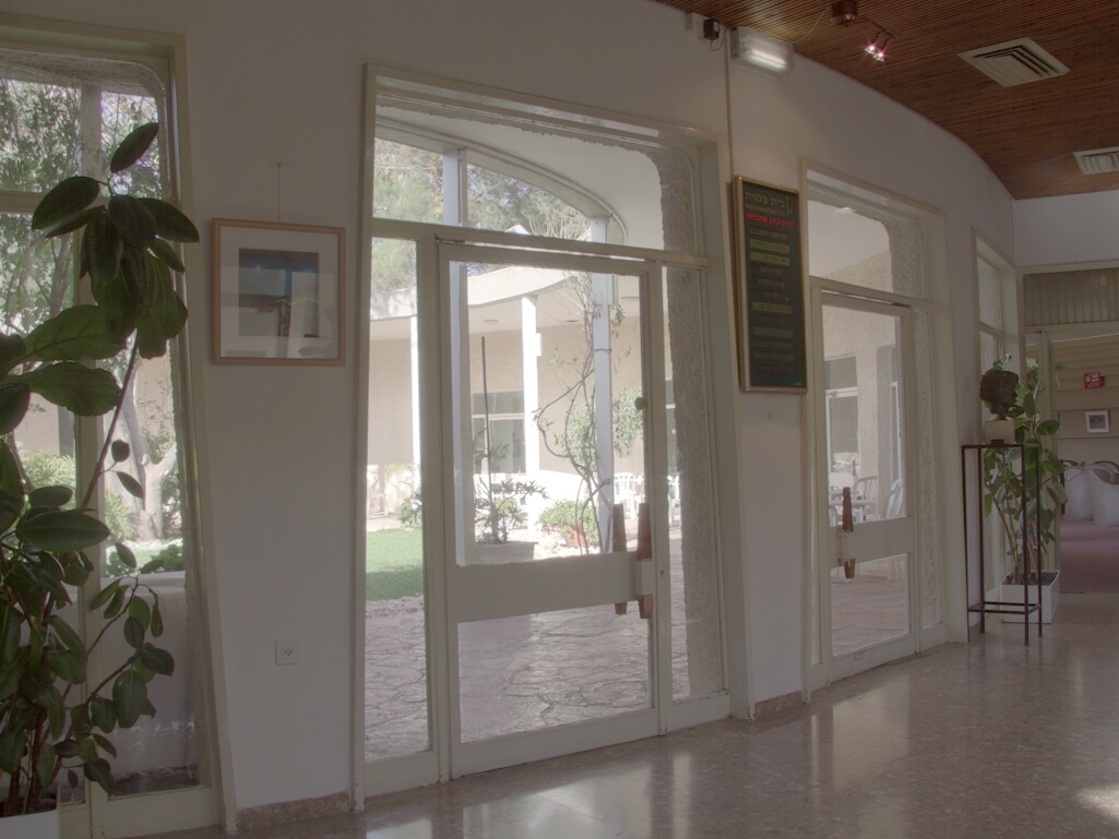
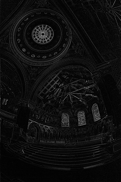
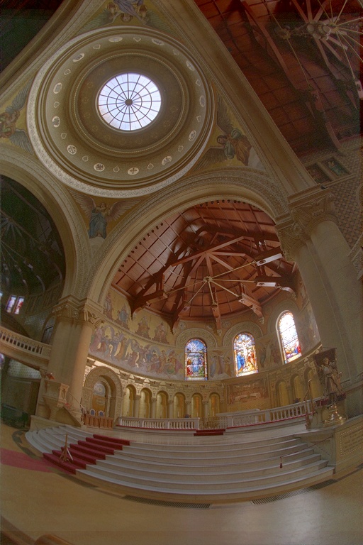
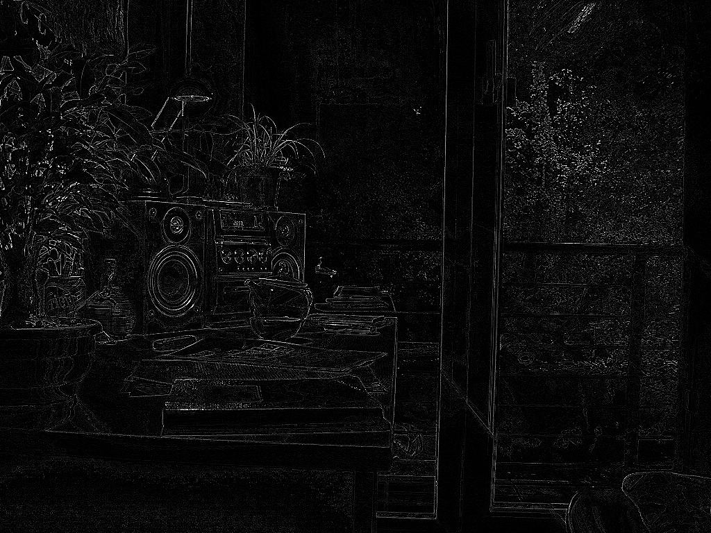
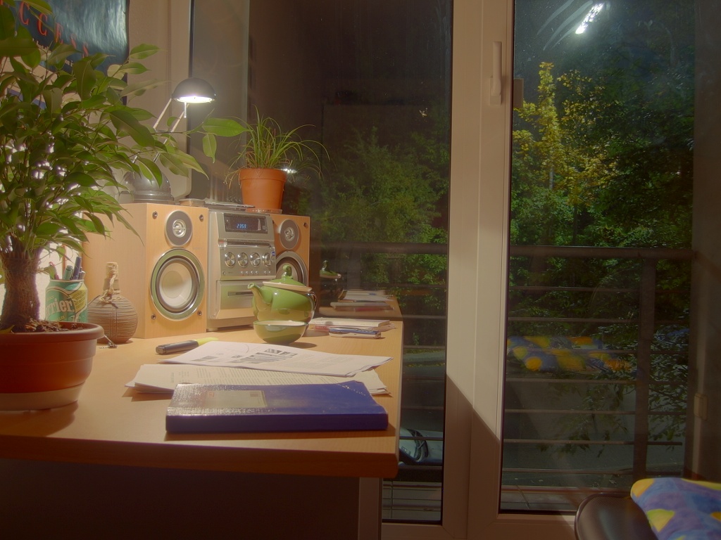
To improve the tone mapping results, more delicate algorithms are needed. Here we use a local tone mapping algorithm, referring to [Fast Bilateral Filtering for the Display of High-Dynamic-Range Images], which uses a bilateral filter to reduce noises and computes a detail layer to better keep the edges. We can see that the results are generally better than those of global tone mapping.

Detail Layer	Local Tone Mapping Result	Global Tone Mapping Result

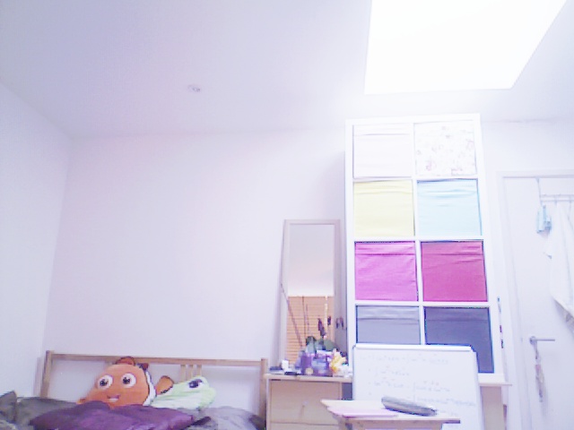
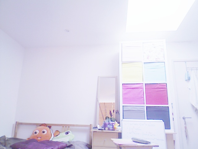
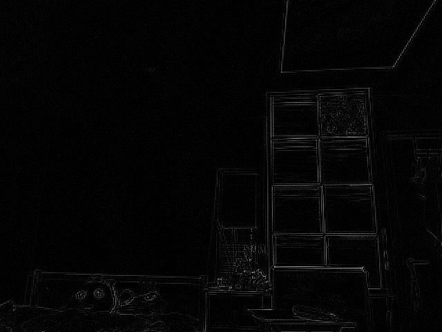
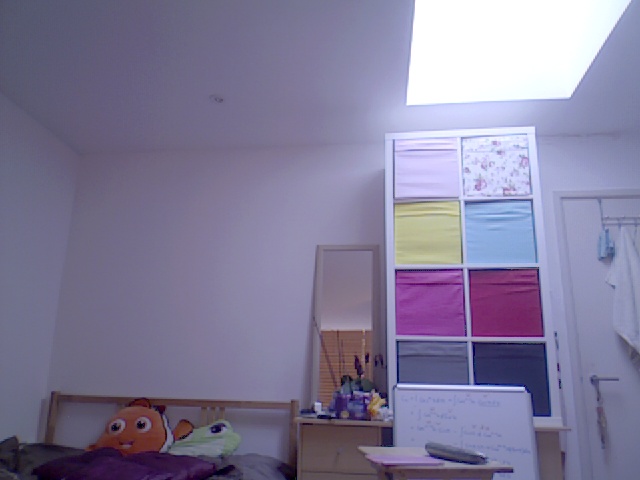
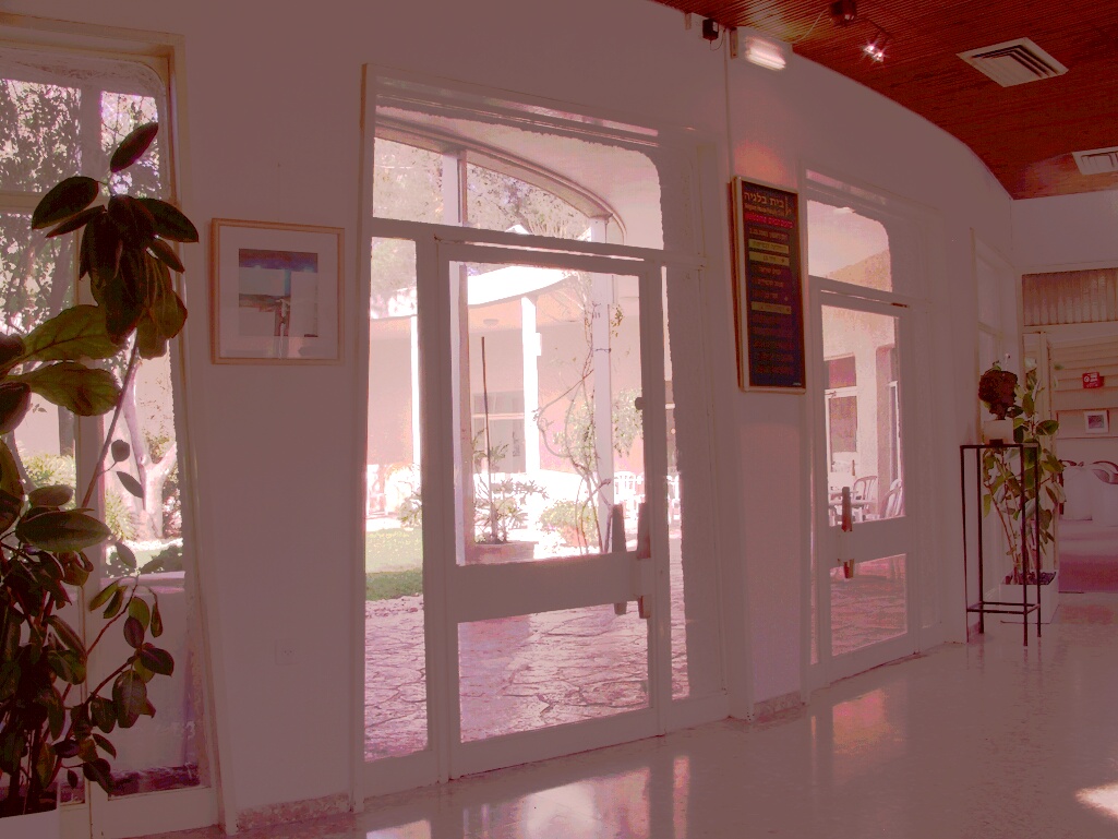
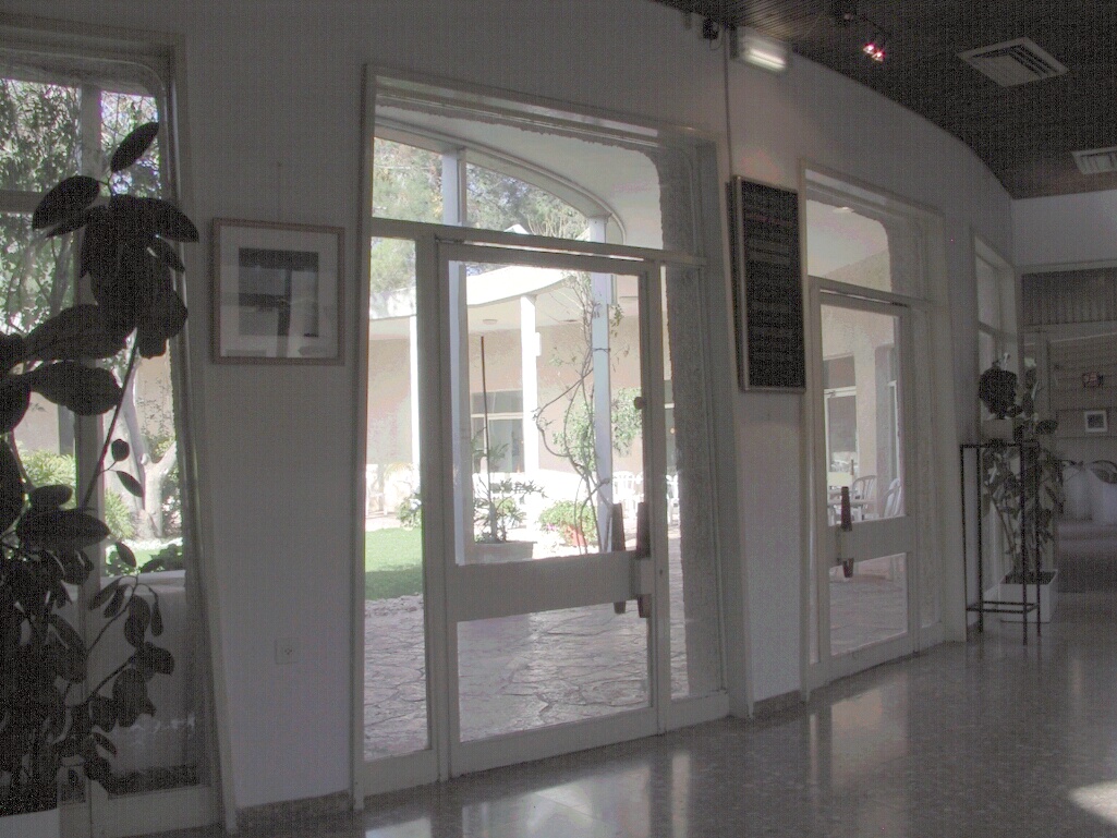
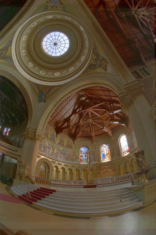
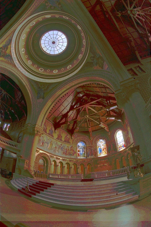
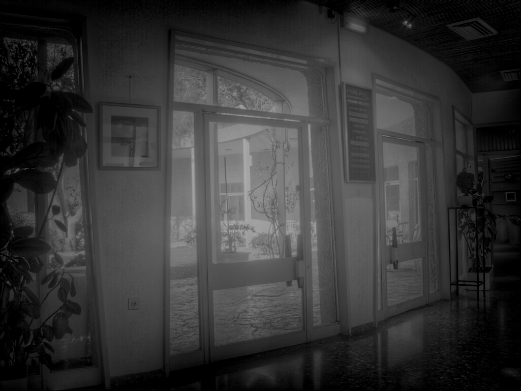
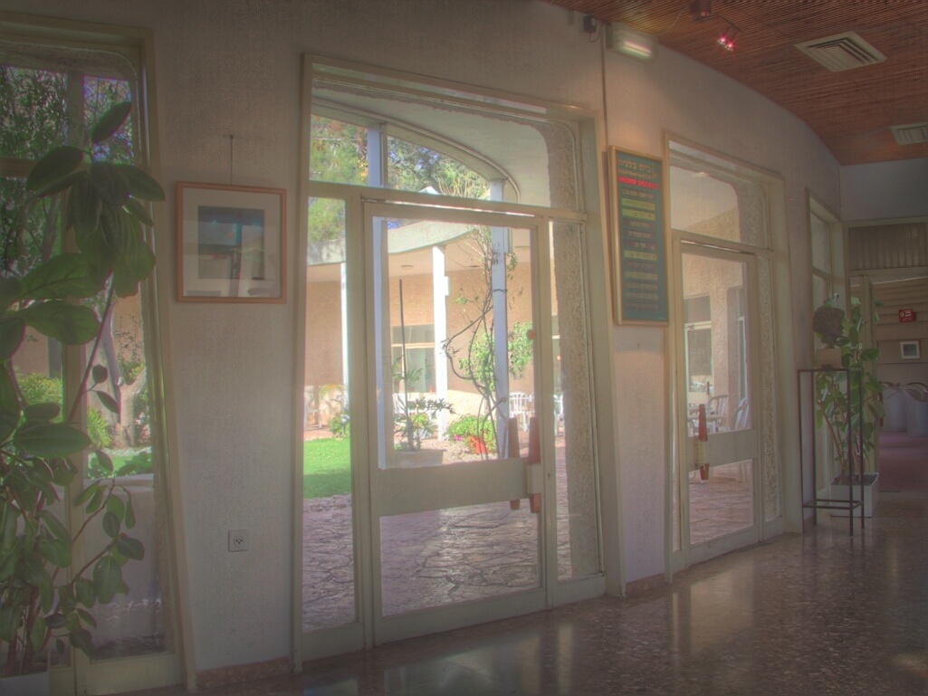
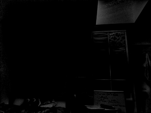
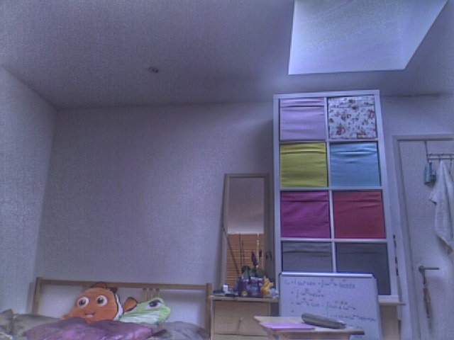
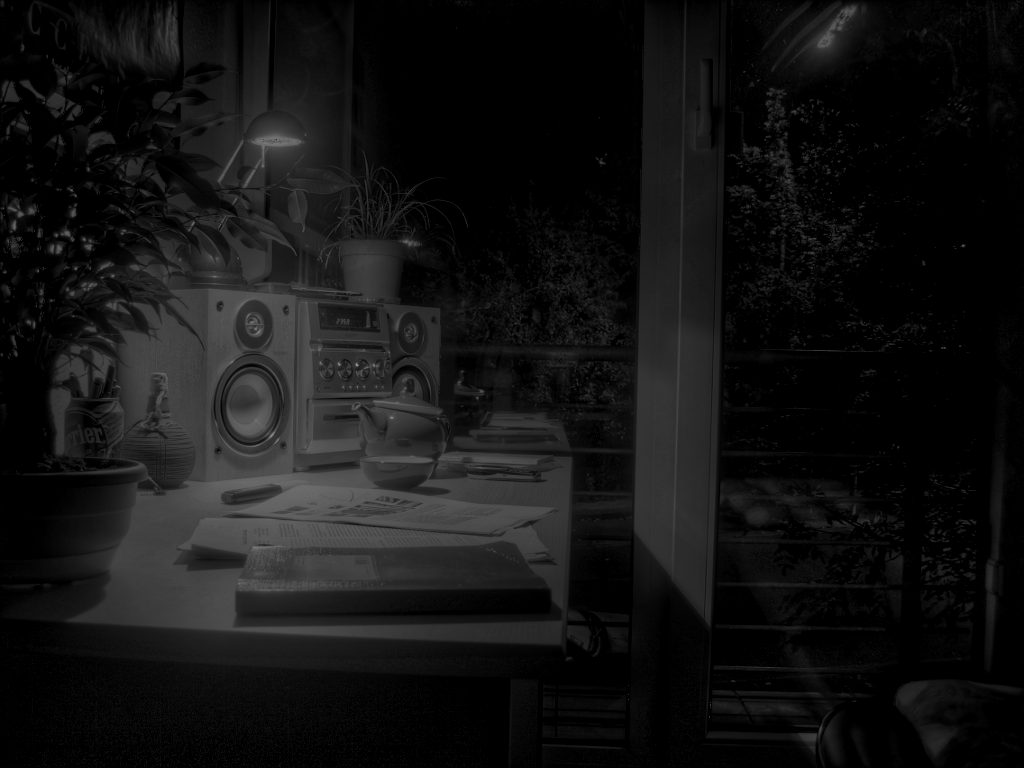
Here are more examples. In these examples, the reults of global tone mapping looks darker, instead of brighter. It may be due to the original image are dark, intead of bright, roughly speaking. But still, results of local tone mapping present more details in a better way.

Detail Layer	Local Tone Mapping Result	Global Tone Mapping Result

Among results generated above, it's not that stable, sometimes one channel of R/G/B in result image will be more obvious, leaving the whole image too 'red' or 'green'. To further improve the results, we calculate the intensity using linear combination of R/G/B channels instead of simply averaging them. Here are the comparisons. First of all, the results become more stable. And we can see that in some cases, it really works and the result looks better.

Results with Average Intensity	Results with Linear Combination of Intensity

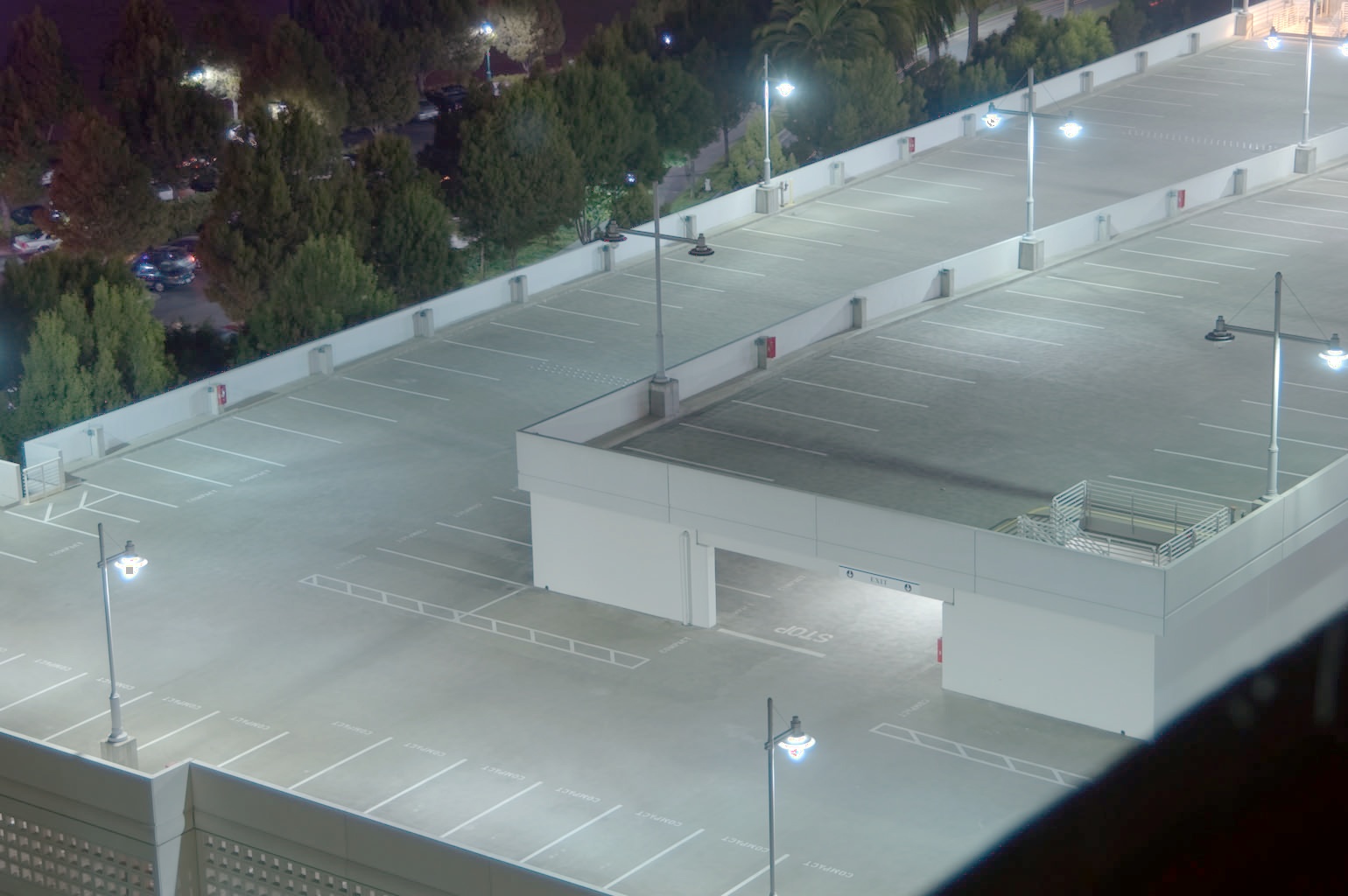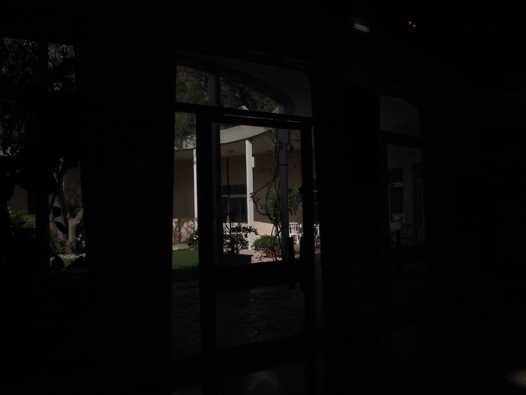
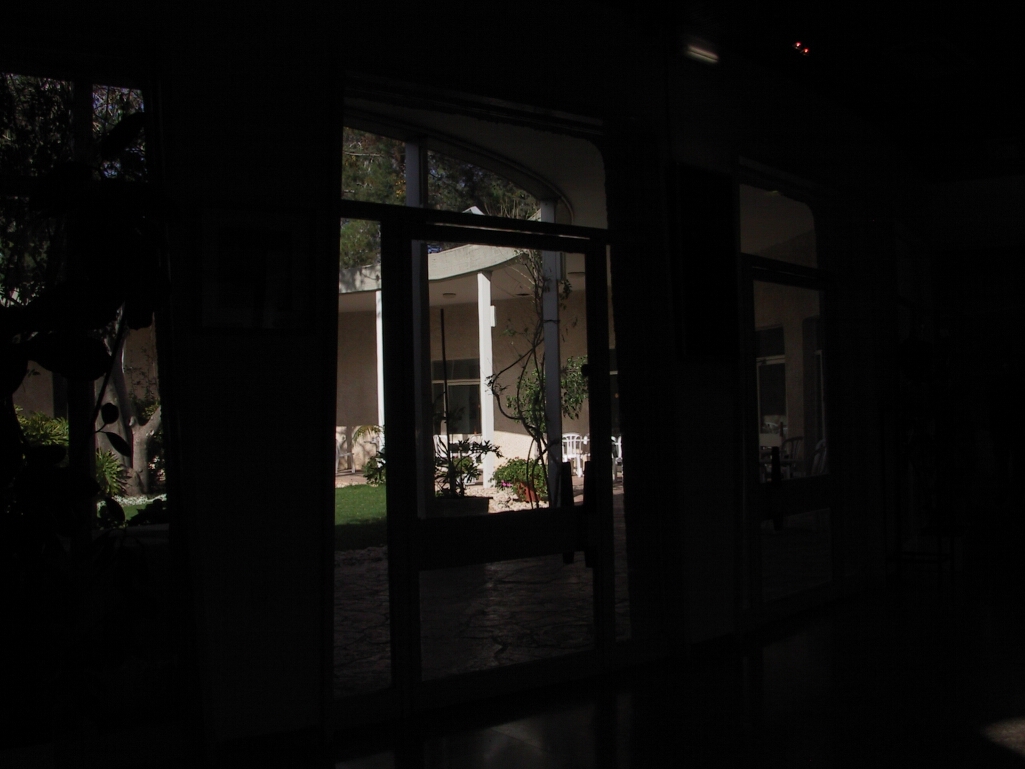
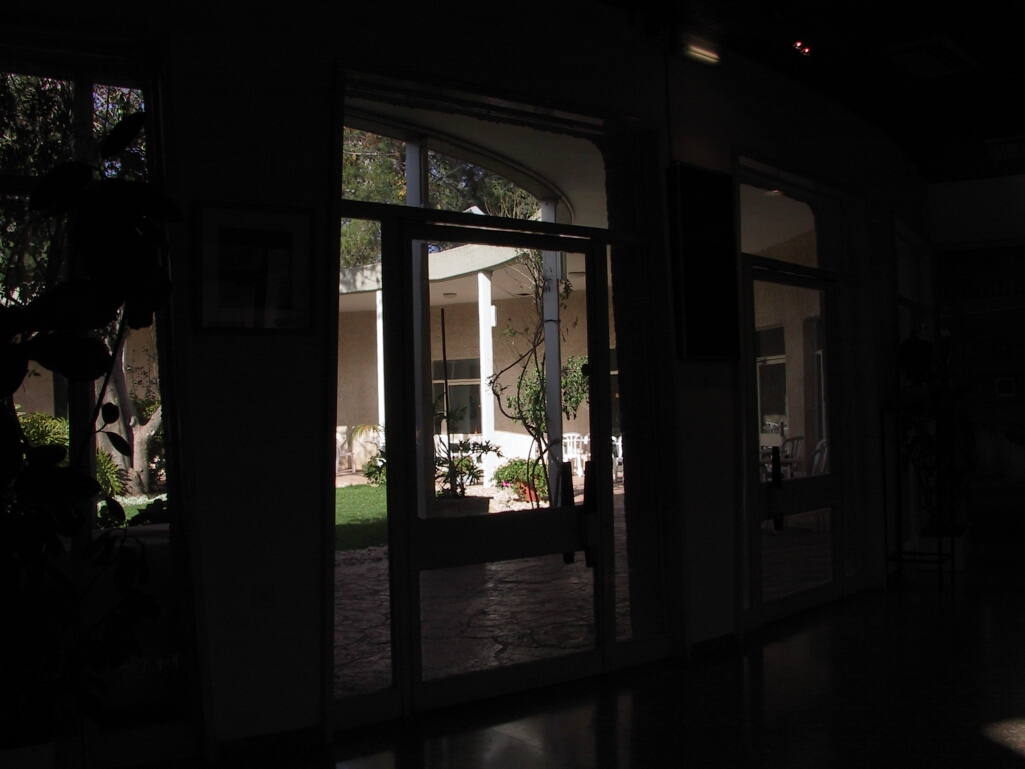
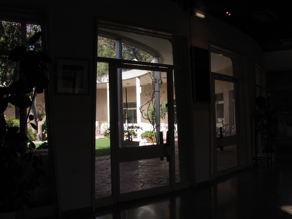
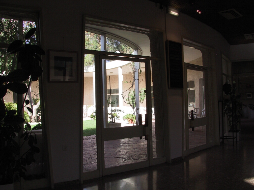
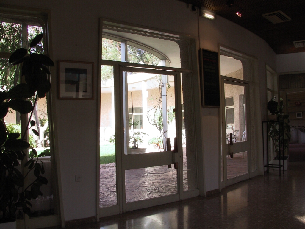
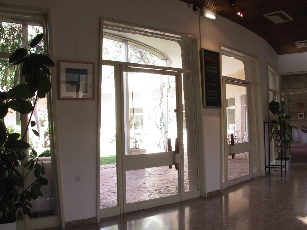
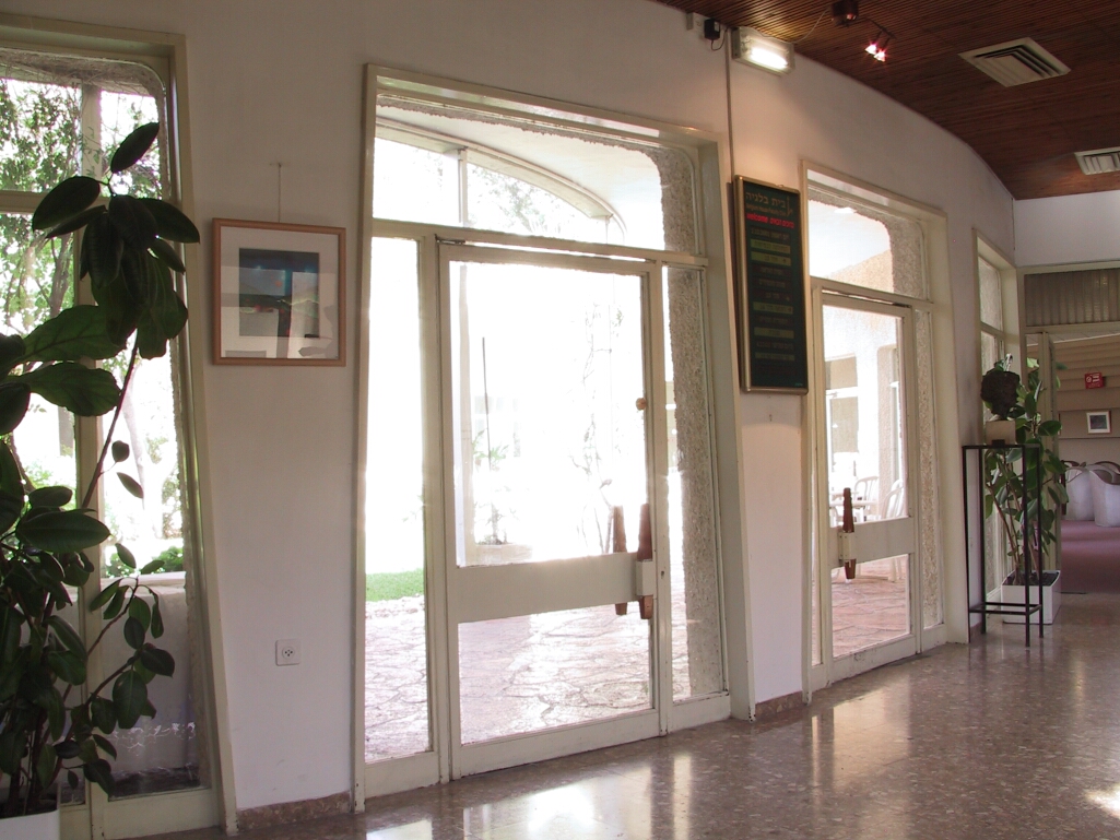
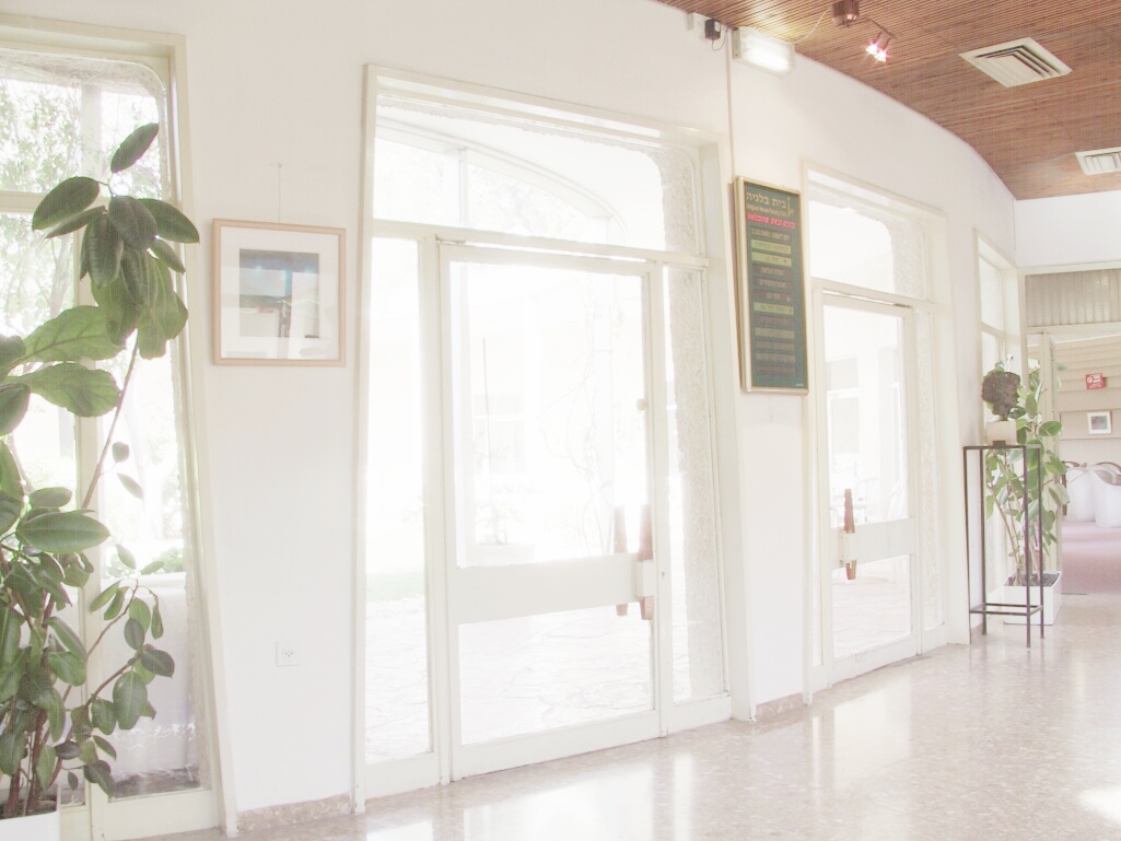
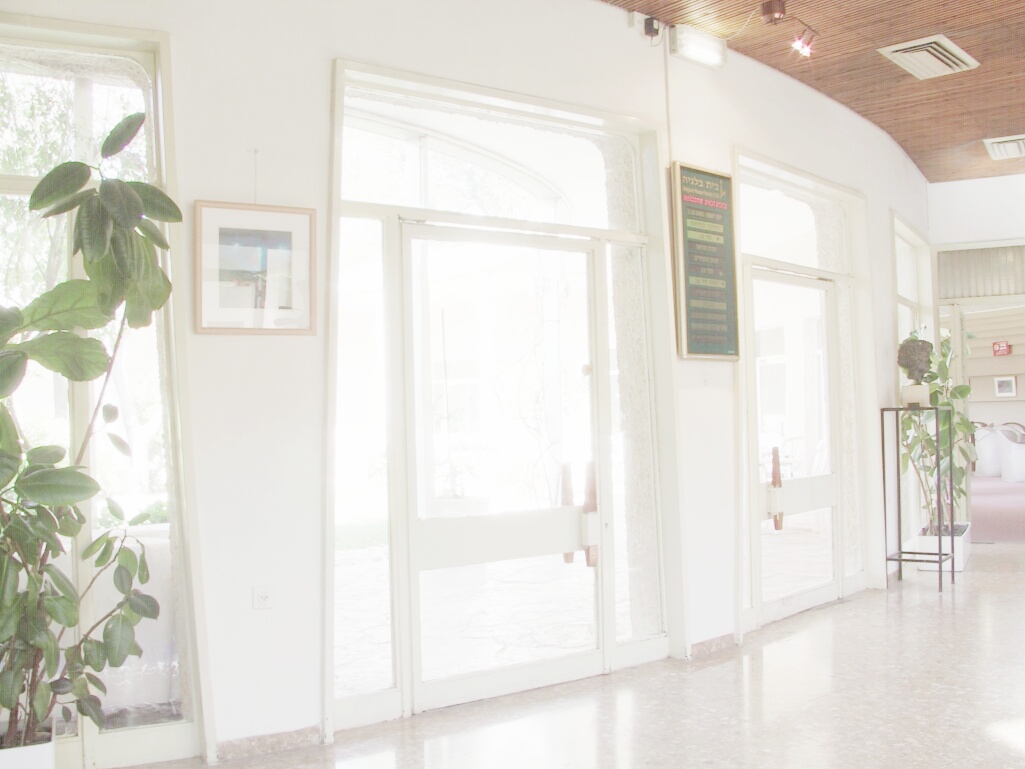
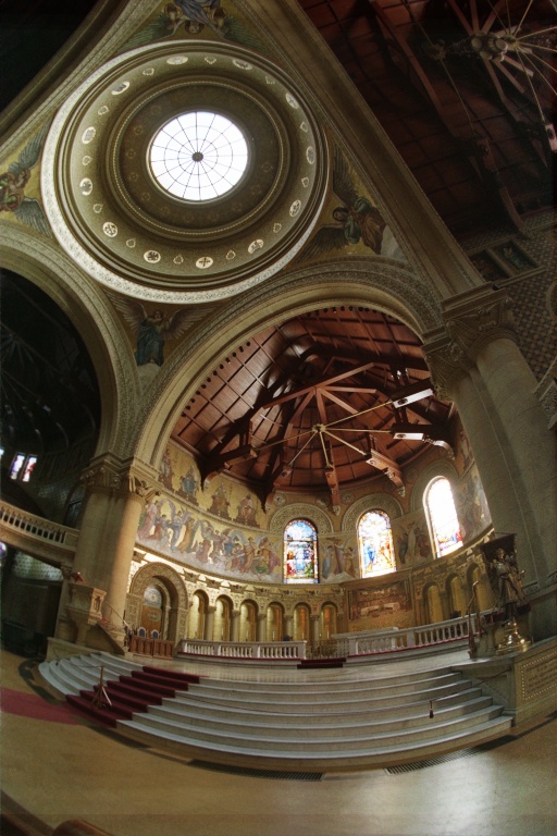
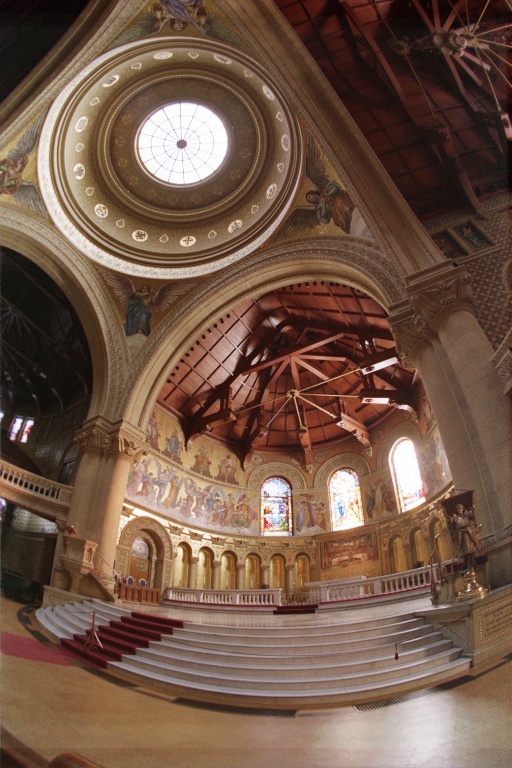
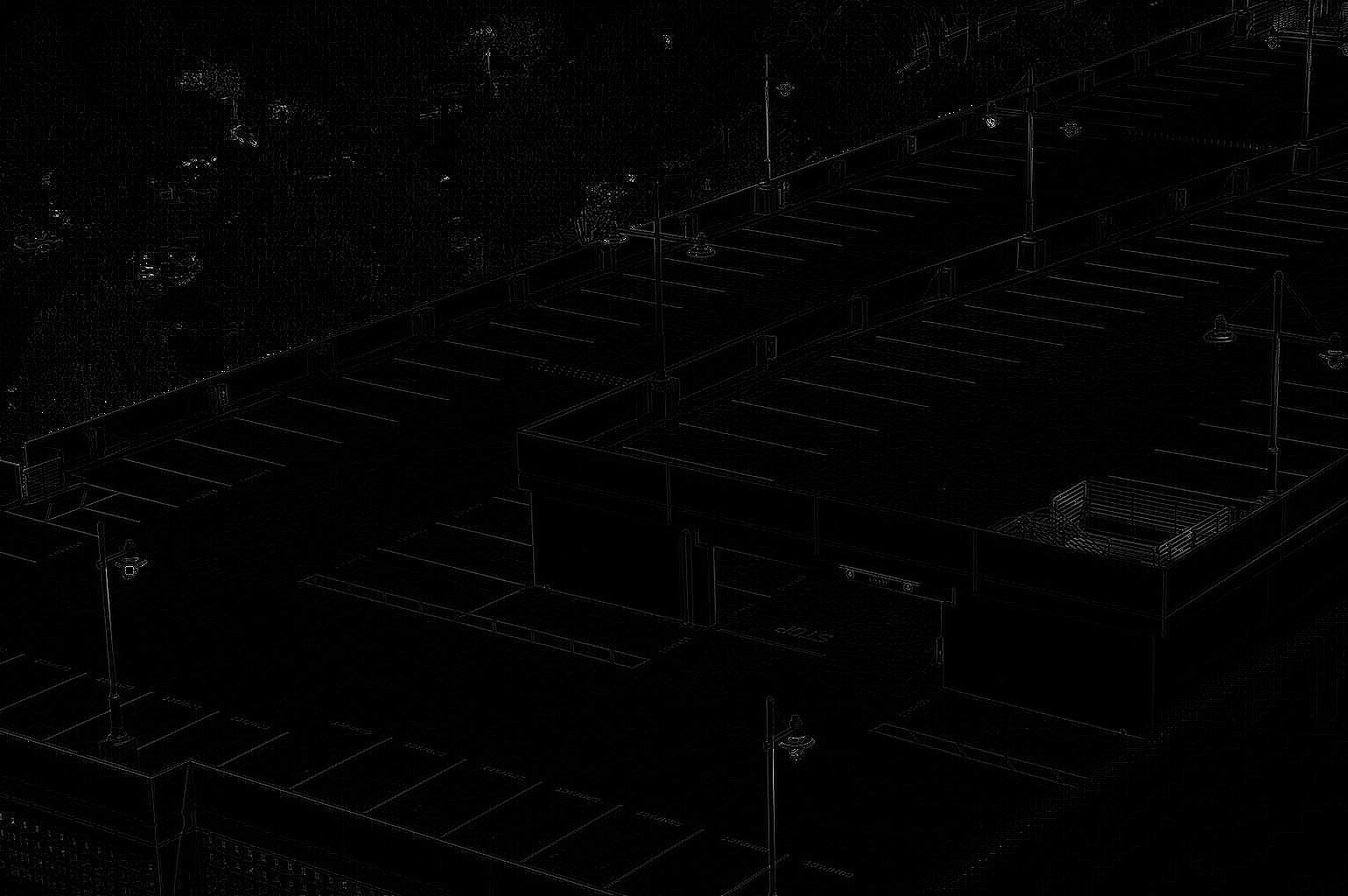
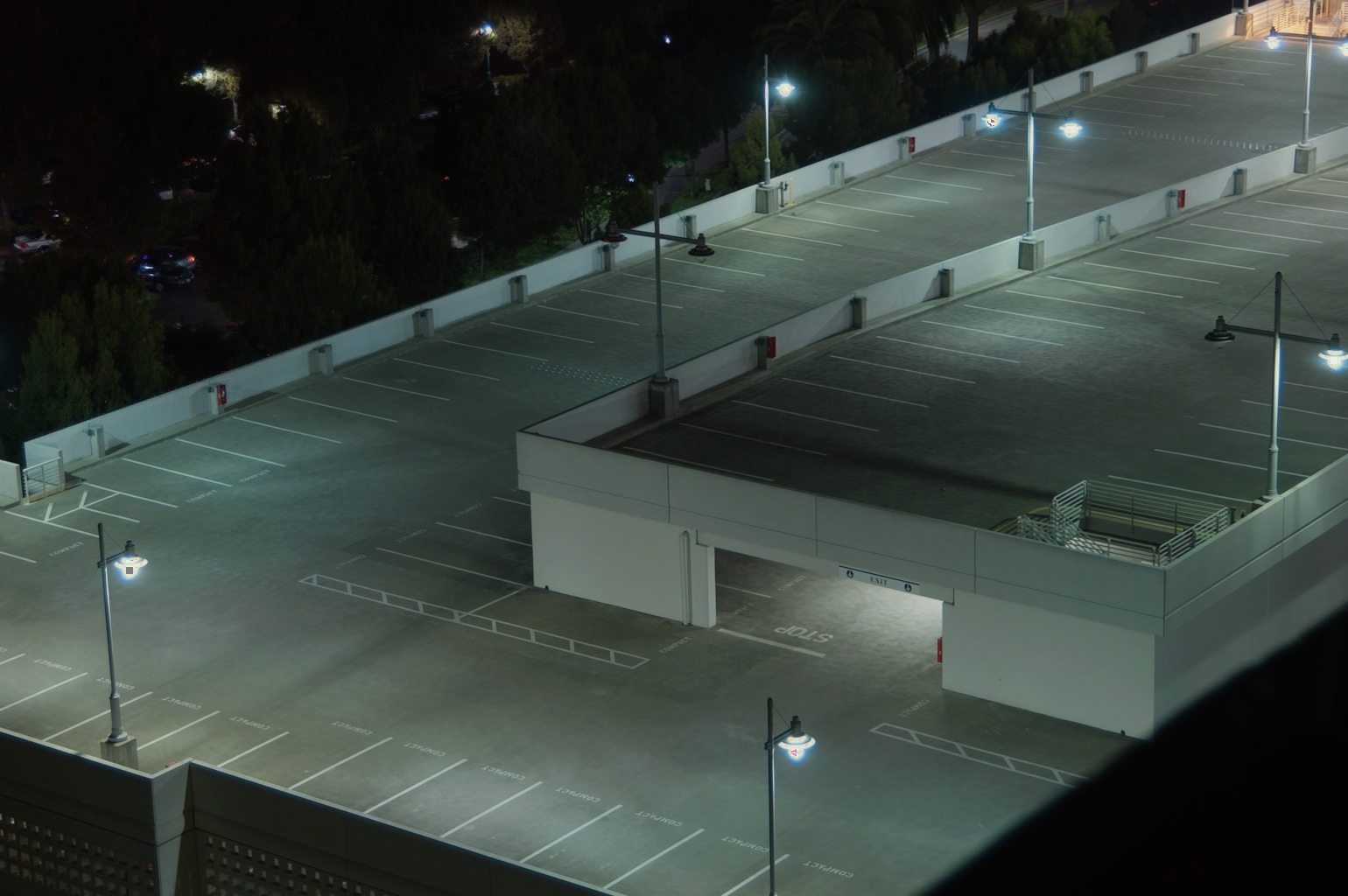
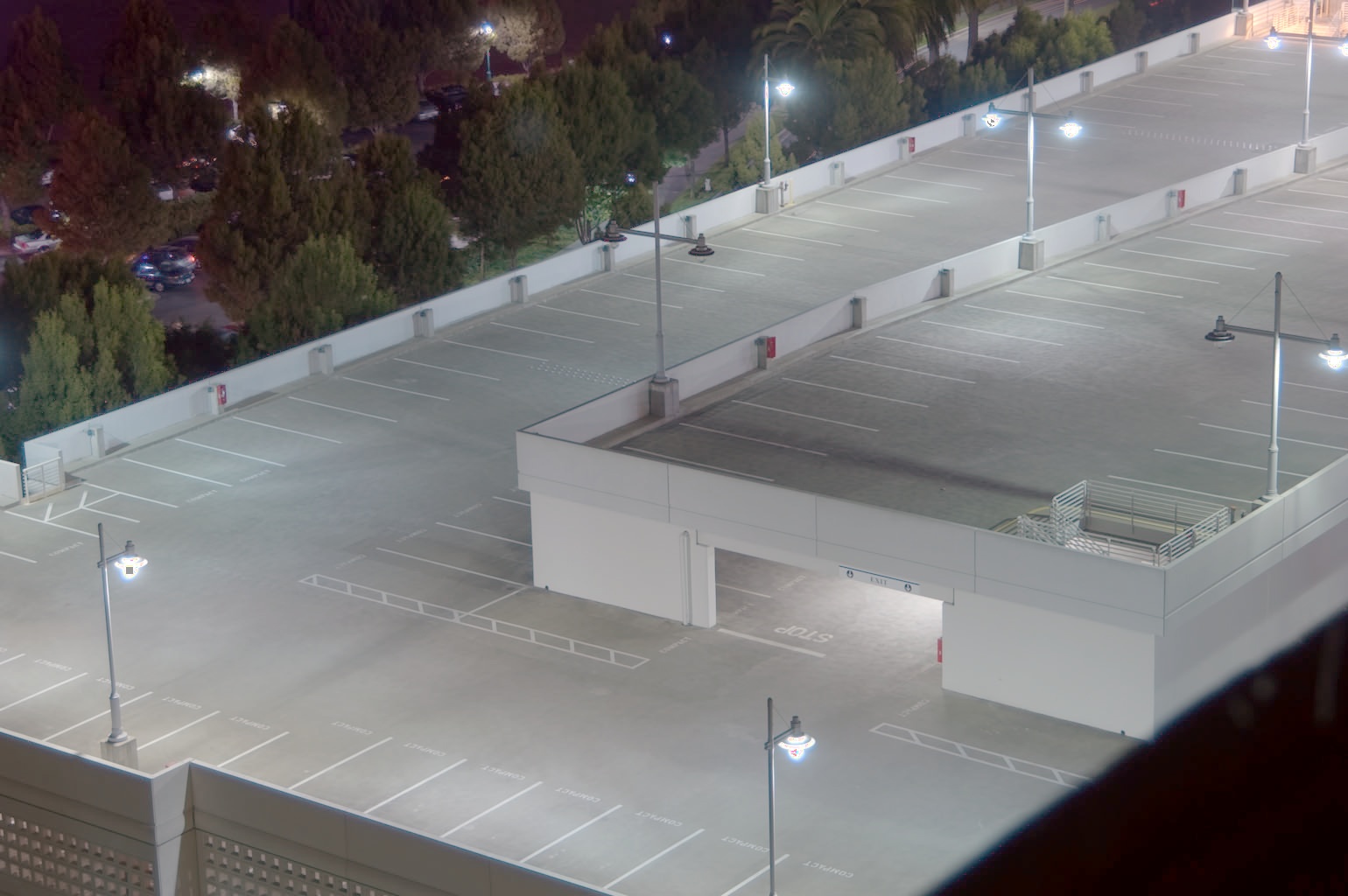
In discussion above, the results are generated based on a whole sequence of source images under different exposures. Afterwards, we re-construct the HDR image by using part of the source images. Here, we sort the images based on exposure time, and then generate the HDR image based on No. 1/3/5/7/9 images (1/2 images), No. 1/5/9 images (1/4 images), No. 1/2/3/4/5 (darker 1/2), No. 3/4/5/6/7 (middle 1/2) and No. 5/6/7/8/9 (bright 1/2) respectively. We can see that if we choose images evenly, the result of 1/2 images still looks quite good. But if we further choose fewer images, the result looks horrible as the radiance map can't be well recovered. And if we choose darker/brighter 1/2 images, the result will look darker/brighter. Besides, if we choose middle/brighter images, there will be some pixels information missing, as those pixels can only be seen clearly in darker images.

Use All Images	Use 1/2 Images	Use 1/4 Images
Use Darker 1/2 Images	Use Middle 1/2 Images	Use Brighter 1/4 Images

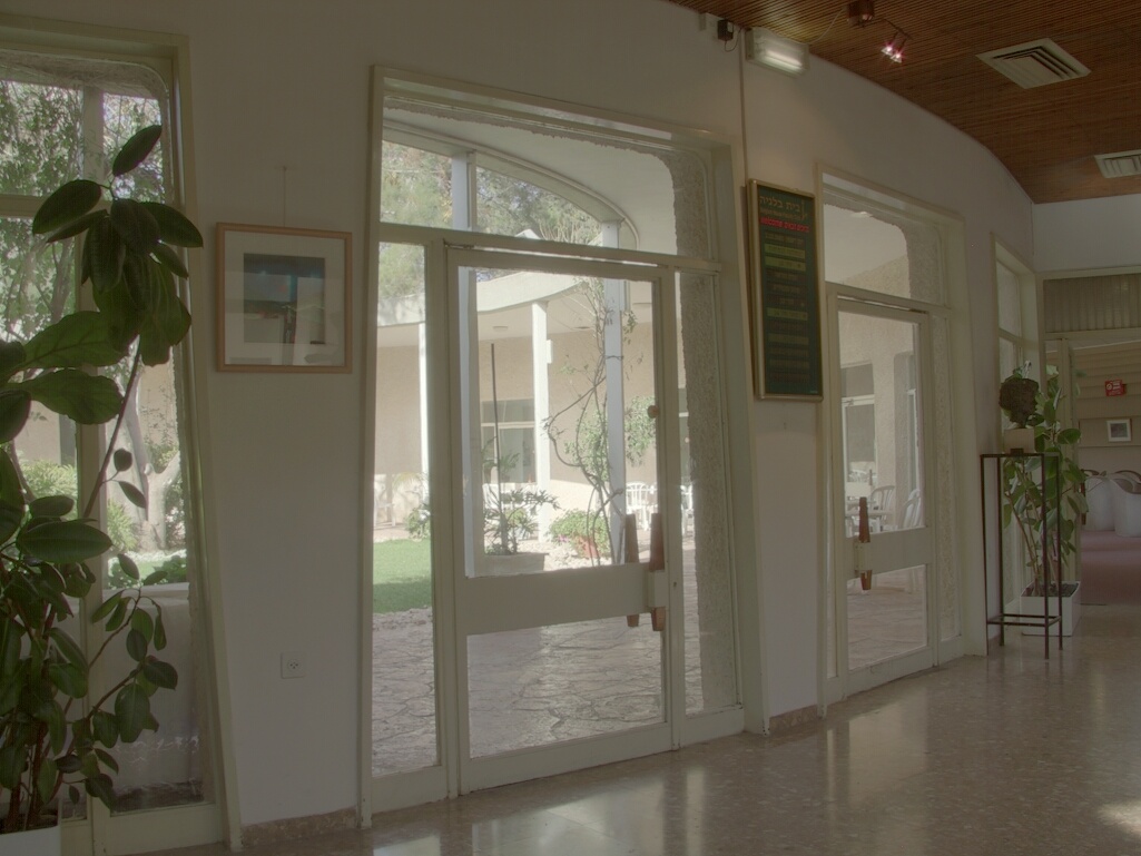
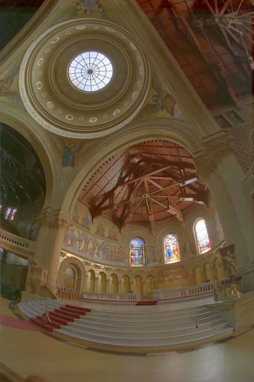
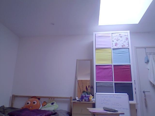
Similarly processing other sets of source images, we get similar results.

Use All Images	Use 1/2 Images	Use 1/4 Images
Use Darker 1/2 Images	Use Middle 1/2 Images	Use Brighter 1/4 Images

Use All Images	Use 1/2 Images	Use 1/4 Images
Use Darker 1/2 Images	Use Middle 1/2 Images	Use Brighter 1/4 Images

Actually, we also implement another local tone mapping algorithm, referring to [Recovering High Dynamic Range Radiance Maps from Photographs], which atteunes the gradients for each pixel to compress the intensity for whole image so that the radiance value can be mapped to a smaller interval, i.e. [0, 255]. Basically, it creates a Gaussian pyramid for the radiance values to keep the ridges information and atteune largely for pixels with larger gradients but relatively slightly for pixels with smaller gradients. However, we didn't obtain quite satisfying results by this method, due to not good enough implementation.

Compressed Intensity	Local Tone Mapping II Result

Both of global tone mapping and local tone mapping are pretty fast. The running time for whole process is around 2 seconds, varying with the actual size of images and the number of images as well as some paramters in code. Actually, here we use matrix to complete many computations, which accelerates the program quite a lot. Previouly, intead of using matrix, using for-loop to calculate, the running time is roughly around 40 seconds, most of which are spent on calculating the real radiance values for all pixels. But for local tone mapping II, it's slower, costing us around 50 seconds or even longer.